Two Dimensional Periodic Systems: Part I

Lattices and Translational Symmetry

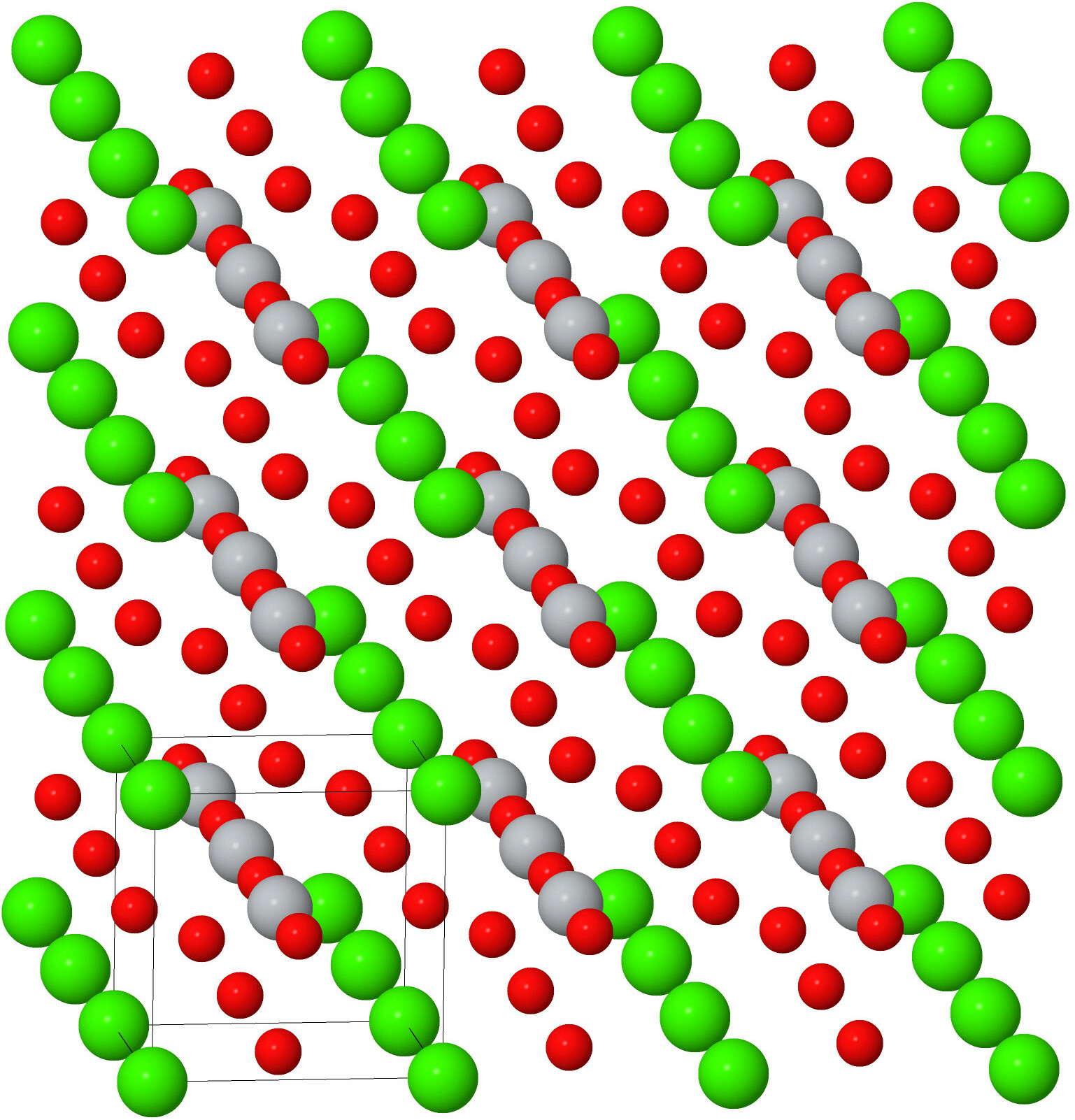
Solid materials are often found as crystals – three-dimensional periodic arrays of atoms. One example of this is cubic perovskite, shown in Fig. 1. The calcium (green) atoms form a cube. Inside the cube is a titanium atom, and on the faces are oxygen atoms. We form the crystal when we stack the cubes together. You can also see the periodicity by drawing a line that passes through any two calcium (green) atoms: you’ll find that the line contains an infinite number of calcium atoms, equally spaced. A line through any pair of titanium (gray) or oxygen (red) atoms will produce a similar result. This periodicity is the heart of crystallography. Here we’ll discuss some of the basics of crystallography – unit cells, primitive vectors, and basis vectors.

Cubic Perovskite Structure — Figure 1: Crystal structure of cubic perovskite, CaTiO₃. The green atoms are calcium, gray atoms titanium, and red atoms oxygen. The small cube outlined at the front lower left of the picture is the unit cell (defined below) of the system.

The Lattice

While the crystals we’re usually interested in are three dimensional objects, periodic systems can exist in any n-dimensional space, in particular in two dimensions. Since it is easier to discuss 2-d objects in a 2-d medium we’ll start with n = 2, but everything we talk about will carry over to three dimensions, which we’ll cover in a later discussion.

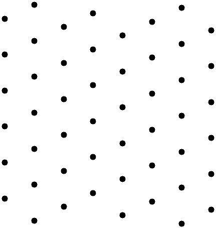
All crystal structures are based on the lattice, a periodic array of points in n-dimensions. A sample 2-d structure lattice is shown in Fig. 2.

Two Dimensional Lattice — Figure 2: A finite portion of a two dimensional lattice.

From this figure we get a couple of properties of periodic systems:

Just as with perovskite, a line drawn through any two lattice points will intersect an infinite number of other lattice points, all evenly spaced on the line.
This system has translational symmetry: we can choose the origin as any point on the lattice. Moving the origin from one point on the lattice to another doesn’t change anything about how we view the crystal.

The translational symmetry of the lattice is discrete: we can only move the origin from one lattice point to another. This limited set of translations can be described with a set of primitive vectors, n of them for a n-dimensional lattice. shows one choice for the primitive vectors in our sample lattice. Once we have the primitive vectors and a starting point all points on the lattice are found at

R = n₁a₁ + n₂a₂ , (1)

for all integers n₁ and n₂.

Two dimensional lattice plus
primitive vectors — Figure 3: The lattice from Fig. 2 with the primitive vectors (1). The vectors plus the blue lines outline the unit cell of the system.

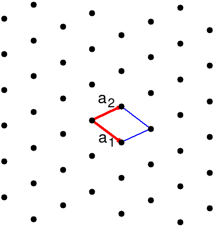
Figure also shows a parallelogram. This is a possible unit cell of the lattice. Think of it as a piece in a very boring jigsaw puzzle. We create the lattice by packing the identical puzzle pieces together, with the lattice points at the intersections. A unit cell is the smallest possible piece that reproduces the lattice.

Once we know the primitive vectors for lattice we can find the area of the unit cell. If our vectors have the Cartesian coordinates

$\begin{array}{cccc} \mathbf{a}_{1} & = & a_{1x} ~ \hat{x} + a_{1y} ~ \hat{y} & \mathrm{and} \\ \mathbf{a}_{2} & = &a_{2x} ~ \hat{x} + a_{2y} ~ \hat{y} &, \end{array}$ (2)
then the area of unit cell is
$A = \left| \begin{array}{cc} a_{1x} & a_{1y} \\ a_{2x} & a_{2y} \end{array} \right| = a_{1x} a_{2y} - a_{1y} a_{2x} ~ .$ (3)
Equivalently if $a_{i}$ is the length of vector $\mathbf{a}_{i}$ and the angle between the two vectors is $\theta$ the area of the cell is just
$A = a_{i} a_{2} \sin\theta$ . (4)
By convention the cell is said to be right-handed if $A$ is positive ($0 \lt \theta \lt 180\degree$) and left-handed if it is negative ($-180\degree \lt \theta \lt 0$). We will see a hand-waving justification of these names when we look at three dimensional lattices. In any case it’s only a convention and doesn’t affect the properties of the structure.

There is considerable freedom in defining primitive vectors. The only rules are that a primitive vector must point from one lattice point to another and that the unit cell area (3) stays the same. Mathematically, any two choices of primitive vectors $\mathbf{a}_{i}$ and $\mathbf{a}'_{i}$ are equivalent if

$\left( \begin{array}{c} \mathbf{a}'_{1} \\ \mathbf{a}'_{2} \end{array} \right) = \left( \begin{array}{cc} n_{11} & n_{12} \\ n_{21} & n_{22} \end{array} \right) \cdot \left( \begin{array}{c} \mathbf{a}_{1} \\ \mathbf{a}_{2} \end{array} \right) ~ ,$ (5)
and
$\left| \begin{array}{cc} n_{11} & n_{12} \\ n_{21} & n_{22} \end{array} \right| = \pm 1 ~ ,$ (6)
the last condition conserving the cell area $|A|$.

Possible unit cells for the lattice
generated using different sets of
primitive vectors — Figure 4: Possible unit cells for the lattice generated using different sets of primitive vectors (5). Every choice of primitive cell tiles the entire plane and so represents the same structure.

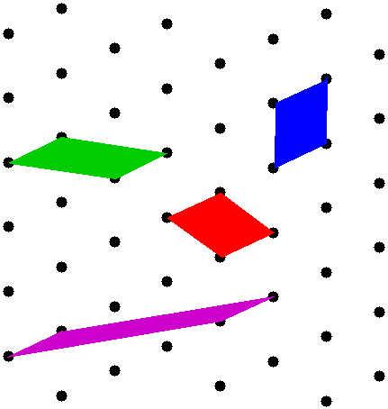
There are an infinite number of possibilities for the unit cell shape, some more practical than others. shows a selection where the unit cells are parallelograms generated by different choices of primitive vectors (5). All these cells describe the same lattice: they all have the same area, and they all tile the plane. Any one of them is an acceptable unit cell.

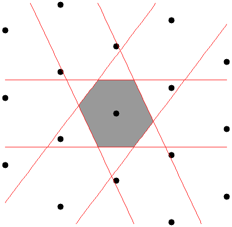
Is there any unique unit cell that we can draw independent of the choice of primitive vectors? At least one such cell exists. It’s called the Wigner-Seitz cell ¹ and it is the set of all points in space that are closer to one lattice point than to any other. The Wigner-Seitz cell for the lattice in is shown in . It was drawn by determining the half-way point between the central lattice point and every other lattice point. Since you can draw this cell around any lattice point it tiles the lattice and makes an acceptable unit cell with the lattice point at the center of the cell.

Figure 5: The Wigner-Seitz cell for the lattice in Fig. 4. The red lines are half-way between the central lattice point and each of the neighboring lattice points. The shaded space is the collection of all points that are closer to the central lattice point than to any other lattice point, defining the cell.

Decorating the Lattice – The Basis

While all this talk of lattices, primitive vectors, and unit cells are useful for defining crystal structures, the lattice shown in is not particularly interesting by itself. A real crystal structure like the one shown in has a lot more going on. To spice up our lattice let’s add two “atoms,” a blue circle and a red circle, to one unit cell in Fig. 2. Since we want a 2-dimensional crystal, all of the cells have to be identical, which means we have to add these atoms in the same place in every unit cell. The result is shown in Fig. 6.

Lattice plus two atom
basis — Figure 6: with the addition of a basis of two atoms. The small black circles are the lattice points from Fig. 2.

Real crystals can from any number of atoms in the unit cell (cubic perovskite, Fig. 1 has five), but we’ll keep it simple here.

It’s important to realize that the red and blue atoms are not lattice points. The blue and red atoms aren’t the same, and they aren’t separated by any primitive vector (2). Instead, they form the basis of the crystal structure. In the real world this is where all the physics and chemistry happen.

Now we have a red atom and a blue atom in each unit cell. Which unit cell? It doesn’t matter. As shown in Fig. 7, any unit cell, no matter how we define it, has exactly two atoms.

Lattice plus basis and
multiple possible unit cells. — Figure 7: The decorated lattice of Fig. 6 showing possible choices for unit cells from Fig. 4 and Fig. 5. Each cell contains exactly two atoms plus the lattice point. In two of the cells the blue atom is near the boundary so that parts of the atom appear on two sides of the cell. This apparent fission is resolved when we periodically repeat the unit cell, joining the bits together.

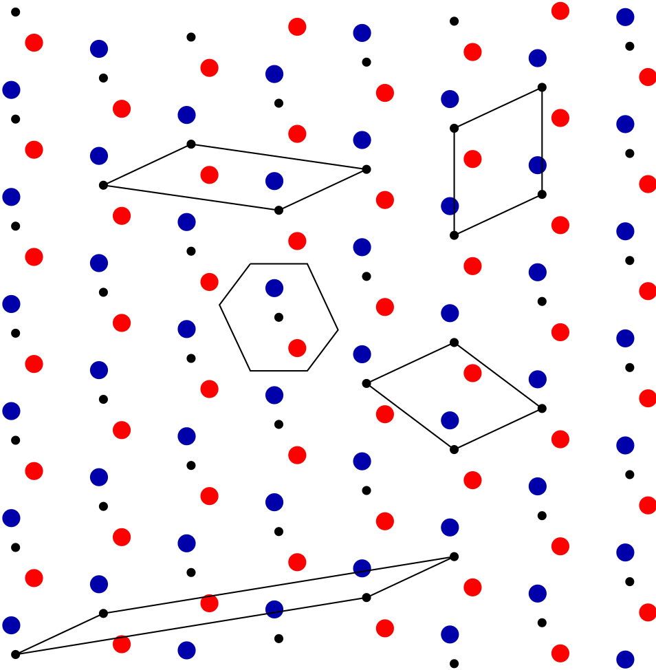
Any of the unit cells in this figure are valid for describing the system. Which one should we use? That will depend on what choice is convenient for the problem at hand.

If we actually want to do anything, such determining the X-ray diffraction pattern of the lattice or performing calculations to determine structure properties, we need be able to tell the rest of the world, including computer programs, about the location of the atoms in the crystal structure. To do this we first have to pick a set of primitive vectors and fix the origin. Then we need to tie down the atoms’ positions by introducing the basis vectors, one for each atom, describing the position of the atoms relative to the origin. These vectors are universally designated as $\mathbf{B}_{i}$, where i designates the atom in the structure. One choice of basis vectors for our structure is shown in Fig. 8.

Lattice plus basis with
primitive and basis vectors. — Figure 8: Close up shot of the decorated lattice shown in , showing the our choice for the primitive vectors $\mathbf{a}_{1}$ and $\mathbf{a}_{2}$ and the basis vectors $\mathbf{B}_{1}$ and $\mathbf{B}_{2}$. The dashed line is the Wigner-Seitz cell for this structure. The choice of basis vectors is not unique, as any vector $\mathbf{B}_{i} + n_{1} \mathbf{a}_{1} + n_{2} \mathbf{a}_{2}$ can be used as a basis vector.

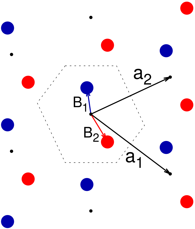
Like nearly everything else we’ve discussed here, the choice of basis vectors isn’t unique. Any vector

$B'_{i} = \mathbf{B}_{i} + n_{1} \mathbf{a}_{1} + n_{2} \mathbf{a}_{2}$ (7)
with any integers $n_{1}$ and $n_{2}$ is a valid choice for the basis vector for atom $i$. Your choice of basis vectors will depend on what you want to do with the structure. Here we chose to keep the vectors inside the Wigner-Seitz cell, but there is no reason we had to.

While we can specify the coordinates of the basis vectors in Cartesian coordinates, it’s often useful to specify the lattice coordinates in terms of the lattice vectors, e.g.

$\mathbf{B}_{i} = \alpha_{i1} \mathbf{a}_{1} + \alpha_{i2} \mathbf{a}_{2}$ , (8)
where the α_ij are the lattice coordinates of the basis vectors. We calculate the coordinates using the reciprocal lattice vectors. These are always $\mathbf{b}_{i}$ (don’t confuse them with the basis vectors $\mathbf{B}_{i}$). They are defined so that
$\mathbf{a}_{i} \cdot \mathbf{b}_{j} = 2 \pi \delta_{ij}$ , (9)
where &delta_ij is the Kronecker delta. The factor of 2π is not particularly important here. We’ll see a use for it when we discuss the reciprocal space for the quantum mechanical description of the system, which will be in a much later article in these tutorials.

If our lattice vectors have the form (2), then the reciprocal vectors are given by

$\begin{array}{cccc} \mathbf{b}_{1} & = & \frac{2\pi}{A} \left(a_{2y} ~ \hat{x} - a_{2x} ~ \hat{y} \right) & \mathrm{and} \\ \mathbf{b}_{2} & = & \frac{2\pi}{A} \left( - a_{1y} ~ \hat{x} + a_{1x} ~ \hat{y} \right) & , \end{array}$ (10)
where Ais the area of the unit cell (3). Then we get the lattice coordinates by applying (9) to (8):
$\alpha_{ij} = \mathbf{a}_{i} \cdot \mathbf{b}_{j}/ (2\pi) ~ .$ (11)
In practice the use of Cartesian coordinates or lattice coordinates for the basis vectors depends on the project. The Encyclopedia of Crystallographic Prototypes gives both Cartesian and lattice coordinates for the basis vectors of each structure.

A Real-World Example: Graphene

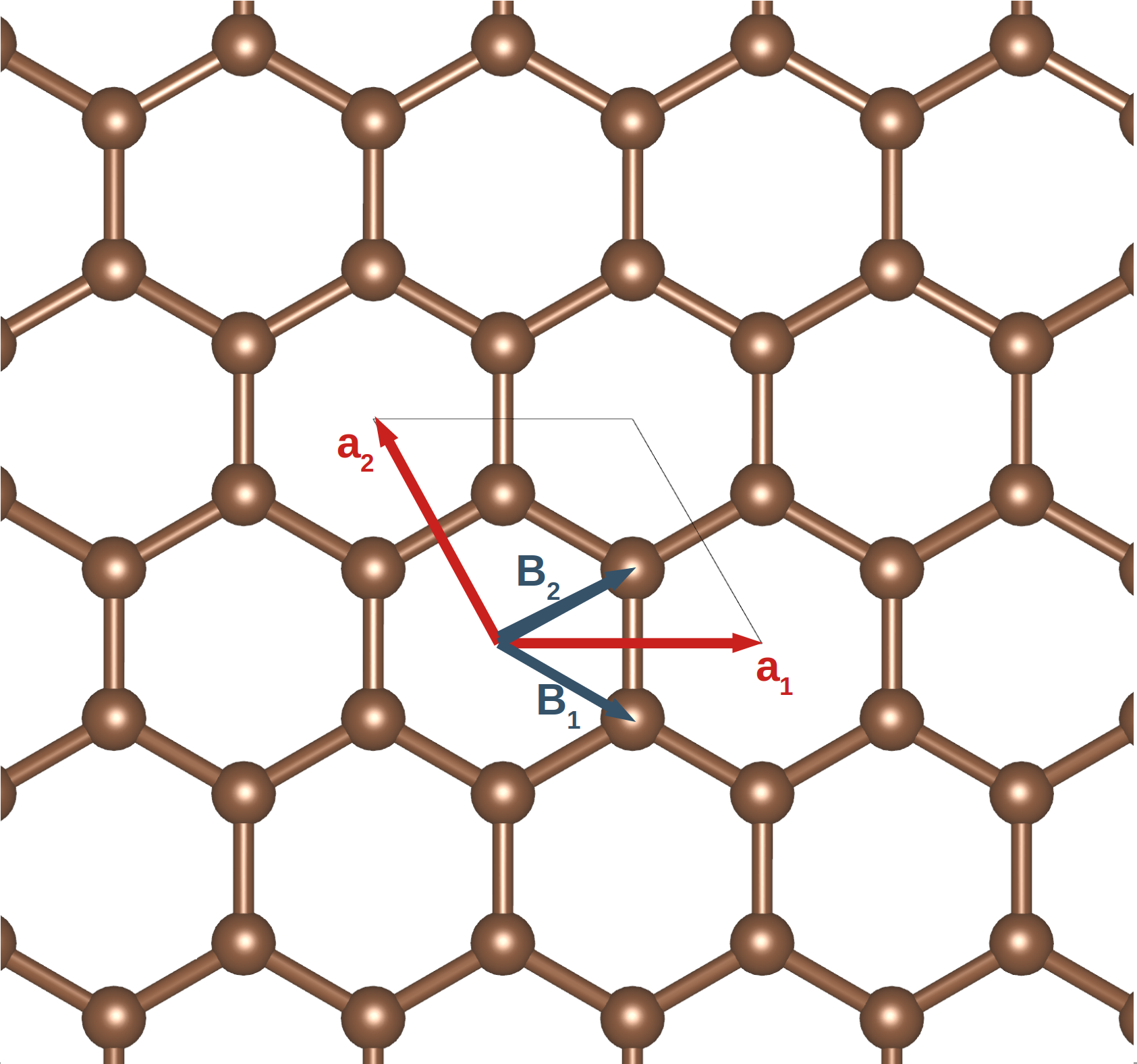
Graphene ² is undoubtedly the most famous two-dimensional crystal structure. It is a single layer of hexagonal graphite, as shown in Fig. 9.

Figure 9: Crystal structure of two dimensional graphene.² The balls show the positions of the carbon nuclei while the lines indicate the bonding between the atoms. The vectors $\mathbf{a}_{1}$ and $\mathbf{a}_{2}$ are the primitive vectors (12), while $\mathbf{B}_{1}$ and $\mathbf{B}_{2}$ are the basis vectors (13) pointing to the distinct atoms in each cell. The parallelogram shows the unit cell determined by our choice of primitive vectors. The Wigner-Seitz cell is the hexagon formed by the ring of carbon atoms. Each carbon atom is part of three Wigner-Seitz cells.

Now that we have a real structure, we can apply the procedures we developed above to describe this system:

The atoms in graphene are arranged in interlocking hexagonal rings. One way to describe this periodicity is to use two primitive vectors of the same length, invariably called a, with a 120° angle between them. Using the alignment of Fig. 9 we’ll set
$\begin{array}{cccc} \mathbf{a}_{1} & = & a \hat{x} & , \\ \mathbf{a}_{2} & = & - \frac{a}{2} \hat{x} + \frac{\sqrt3 a}{2} \hat{y} & , & \end{array}$ (12)
where a ≈ 2.5Å.
The unit cell area (3) is then
$A = \frac{\sqrt3}{2} a^2 ~ . ~$ (13)
The reciprocal lattice vectors (8) are
$\begin{array}{cccc} \mathbf{b}_{1} & = & \frac{2\pi}{a} ~ \hat{x} + \frac{2\pi}{\sqrt3 a} ~ \hat{y} & , \\ \mathbf{b}_{2} & = & \frac{4 \pi}{\sqrt3 a} ~ \hat{y} & . & \end{array}$ (14)
We’ll use the basis vectors drawn in the figure,
$\begin{array}{cccc} \mathbf{B}_{1} & = & \frac{a}{2} ~ \hat{x} - \frac{a}{2\sqrt3} ~ \hat{y} & , \\ \mathbf{B}_{2} & = & \frac{a}{2} ~ \hat{x} + \frac{a}{2\sqrt3} ~ \hat{y} & , & \end{array}$ (15)
or, in lattice coordinates,
$\begin{array}{cccc} \mathbf{B}_{1} & = & \frac23 \mathbf{a}_{1} + \frac13 \mathbf{a}_{2} & , \\ \mathbf{B}_{2} & = & \frac13 \mathbf{a}_{1} + \frac23 \mathbf{a}_{2} & . & \end{array}$ (16)
There are six atoms in any hexagon, but four of them are copies of the other two. The atoms at
$\begin{array}{cccc} \mathbf{B}_{1} + \mathbf{a}_{2} & = & \frac{a}{\sqrt3} ~ \hat{y} & \mathrm{and} \\ \mathbf{B}_{1} -\mathbf{a}_{1} + \mathbf{a}_{2} & = & - \frac{a}{2} ~ \hat{x} - \frac{a}{2\sqrt3} ~ \hat{y} & & \end{array}$ (17)
are periodic replicas of the atom at $\mathbf{B}_{1}$, while the atoms at
$\begin{array}{cccc} \mathbf{B}_{2} - \mathbf{a}_{1} & = & - \frac{a}{2} ~ \hat{x} + \frac{a}{2\sqrt3} ~ \hat{y} & \mathrm{and} \\ \mathbf{B}_{2} -\mathbf{a}_{1} - \mathbf{a}_{2} & = & - \frac{a}{\sqrt3} ~ \hat{y} & & \end{array}$ (18)
are replicas of $\mathbf{B}_{2}$.
One possible unit cell is the parallelogram drawn on the figure. Another is the Wigner-Seitz cell formed by the hexagons. Each of the six carbon atoms on the hexagons is distributed between three Wigner-Seitz cells.

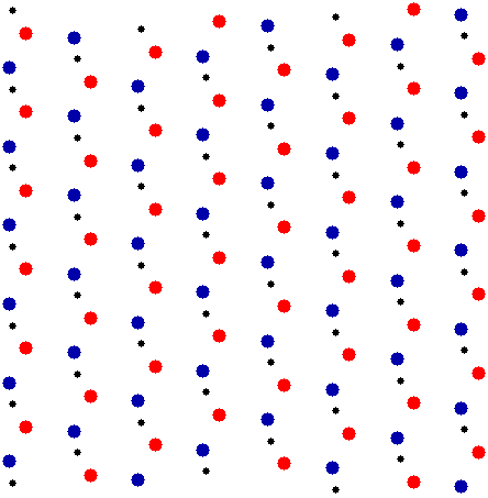
This approach can be applied to any periodic system, not just those composed of atoms. For example, suppose we wanted to construct a periodically repeated series pictures based on the lattice in . The basis vectors of this structure would point to the individual pixels in the digitized image. We then assign a color to each pixel, just as we did in our red/blue “atomic” description. The result might look like Fig. 10. For obvious reasons this type of tiling is called a wallpaper.

Duke Blue
Devel Wallpaper. — Figure 10: A two dimensional periodic tiling (wallpaper) of a college mascot.

More Symmetry

So far we’ve only discussed translational symmetry in the lattice. Graphene (Fig. 9) obviously has much more symmetry than that. For example,

Rotating the structure by 60°, or any multiple of 60°, around the origin,
“Inverting” the atomic positions ($x \leftrightarrow -x$ and $y \leftrightarrow -y$) for all atomic coordinates
Reflecting all the atoms through the y axis ($x \leftrightarrow -x) or the x axis ($y \leftrightarrow -y$),
Reflecting the atoms through a line running through the midpoint of the bonds, or
Reflecting the atoms through a line running through a set of bonds,

will not change what the picture looks like. We’ll discuss these higher symmetries in the next article.

Glossary

Here is a brief definition of some of the terms used in this article:

Basis:: The collection of items (atoms, pixels, paint drops) that decorate a lattice to produce a crystal or a wallpaper. Every object in a crystal structure is part of the basis.
Basis Vectors:: The vectors pointing from the origin of the lattice to the individual members of the basis.
Cartesian (Basis) Coordinates:: The positions of the basis vectors relative to the origin given on a standard Cartesian grid.
Crystal:: A periodically repeated collection of objects in n-dimensions.
Lattice:: A periodically repeated collection of points in n-dimensions.
Lattice Coordinates:: The positions of the basis vectors expressed relative to the chosen primitive vectors of the system.
Primitive Vectors:: A set of vectors that defines the allowed shifts in the origin of the lattice that do not violate translational symmetry.
Reciprocal Lattice Vectors:: A set of vectors forming the “reciprocal space” of the lattice. Here we only use them to determine the lattice coordinates of the basis vectors. There are many more uses for reciprocal lattice vectors which we will discuss in later articles.
Translational Symmetry:: A shift of the origin of a lattice that produces a lattice indistinguishable from the original lattice.
Unit Cell:: The (non-unique) smallest area (smallest volume in three dimensions) of space that reproduces all of the information about the crystal structure, and which can be periodically tiled to create the entire structure.
Wallpaper:: A two dimensional periodically repeated system. A wallpaper may be a collection of atoms, pictures, or abstract designs, so long as they are periodically repeated.
Wigner-Seitz Cell: A uniquely defined unit cell consisting of all spatial points closer to a given lattice point than to any other lattice point.

References

N. W. Ashcroft and N. D. Mermin, Solid State Physics (Saunders College Publishing, Orlando, 1976), chap. 4, pp. 73–75.
A. K. Geim and K. S. Novoselov, The rise of graphene, Nat. Mater. 6, 183–191 (2007), doi:10.1038/nmat1849.
M. J. Mehl, D. Hicks, C. Toher, O. Levy, R. M. Hanson, G. L. W. Hart, and S. Curtarolo, The AFLOW Library of Crystallographic Prototypes: Part 1, Comput. Mater. Sci. 136, S1–S828 (2017), doi:10.1016/j.commatsci.2017.01.017.
D. Hicks, M. J. Mehl, E. Gossett, C. Toher, O. Levy, R. M. Hanson, G. L. W. Hart, and S. Curtarolo, The AFLOW Library of Crystallographic Prototypes: Part 2, Comput. Mater. Sci. 161, S1–S1011 (2019), doi:10.1016/j.commatsci.2018.10.043.

Encyclopedia of Crystallographic Prototypes